

TL;DR
I modeled grocery blueberry ordering as a partially observable Markov decision process and compared a range of observation scenarios - from basic sales and delivery records to Sunrise 2027-style lot-level GTIN codes and temperature histories. Richer data clearly improves freshness beliefs, but not store profit, probably because my controller is too simplistic to leverage the sharper beliefs.
If you don’t want to read a math paper, scroll down to enjoy some pretty graphs, or play with the simulator by clicking on the banner above.
If you’re looking for a challenge, try to beat my ordering policy in the Build-Your-Own-Controller Notebook.
Introduction
Hi friends,
For the last few weeks, I’ve been thinking a lot about blueberries - specifically, the math involved in advising grocery stores on perishable ordering decisions using the data they have available. My initial inspiration was this blog post from Afresh, a data science company that builds software for large US grocers like Albertsons and Meijer, to help them make data-driven inventory decisions, especially in the fresh department, where inventory management is quite complex due to the short shelf-life of fresh food. Their idea is that by making better inventory decisions, we can significantly reduce food waste, which is a huge contributor to climate change. So that’s pretty cool!
In the post, the author, Philip Cerles, paints the picture of a tiny grocery store that only sells two items: cereal and blueberries. He discusses how to decide what to order each day from your supplier, and the additional complexity of choosing the right blueberry order, because if you don’t sell them within a few days, the money you spent on them ends up in the compost pile. That post looks at a very simplified scenario, where you always know exactly how many punnets of blueberries you have, exactly how old each one is, exactly which ones customers will purchase each day, and exactly how long until your berries go bad. Those assumptions let you use Dynamic Programming to efficiently calculate the exact optimal order by looking ahead over a finite horizon.
I see mathematical modeling as similar to linguistic description - you can describe a situation in a few words or a whole book, depending on your goals, and putting anything down on paper requires assumptions that aren’t 100% true. Blueberry ordering piqued my interest, so I’m going to formulate a more complex (and still imperfect) description of it. Additional complexity doesn’t automatically produce better insight, but I hope it sheds light on some interesting new aspects of the situation - and that you’ll enjoy the beauty in the math for its own sake along the way.
Sunrise 2027
As I was researching perishable inventory management, one thing that fueled my curiosity is a major ongoing grocery-industry initiative called Sunrise 2027, which aims to bring 2D barcodes - a GS1 DataMatrix, or a QR code carrying a GS1 Digital Link URI - to the retail checkout alongside the UPC codes we scan today.
The product identifier itself doesn’t change: the UPC and the 2D code carry the same GTIN. What’s new is what a 2D symbol can carry next to it - standardized extra fields called Application Identifiers, the one that matters here being batch/lot number (10). A UPC tells you only what the item is; every pint of blueberries from Sam’s Farm carries an identical one. Add the lot and you get a lot-level identifier - GTIN + lot, written LGTIN - which distinguishes one batch from another batch of the same product from the same farm. Scan that at checkout, and it could be linked to an exact harvest date, and potentially a rich ecosystem of supply-chain data specific to that lot - including storage and transportation conditions, informed by temperature/humidity loggers.
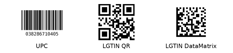
The 2027 date is a capability target, not a mandate - retail point-of-sale should be able to read a GTIN from both linear and 2D barcodes by the end of that year. And the UPC isn’t going away: GS1’s own guidance says linear barcodes “will not go away and will coexist with 2D barcodes for as long as there are uses for them,” with no announced sunset date. So the near-term picture is dual-marked packages and a slowly growing share of checkouts that can read the richer symbol. And while upstream suppliers publishing lot-linked data is on the horizon, the logistics of how will take years to untangle. Here we are, then, looking into the future, offering a small drop of mathematical analysis to the conversation of what might be, and if/how it matters.
Project Overview
In this project, I develop a simple grocery store simulator. It models spoilage physics, shipment conditions, and consumer demand/preferences. The simulator uses these models to generate “true” events/outcomes. Each day, blueberries are ordered, delivered, sold and spoiled according to the simulator’s model.
I also develop a “filter”, which does its best to infer the true state of the system based on partial observations, namely sales, waste counts, and delivery information. We consider several different observation scenarios, representing stores with different procedures/technology for tracking reality. Ultimately, the big question is “what’s on the shelf right now, and how fresh is it?” Notably, the filter uses the same model of reality as the simulator, so although it has imperfect information, it can use its accurate understanding of reality to formulate its beliefs.
Finally, there’s the “controller”, which takes the filter’s beliefs about the current state of the system and uses it to make decisions. Specifically, we’re just focused on one decision: how many blueberries to order.
The heart of the codebase is implemented in Rust, with Python and WASM bindings, allowing the same code to be used in Jupyter notebooks running large calculations in the cloud, as well as in the web-browser on your mobile phone. There’s a fully interactive web UI that allows you to explore the simulator, filter, and controller, tweak simulator parameters, change observation scenarios, and visualize everything. It’s kind of fun ;)
The model
We won’t assume perfect knowledge of inventory. In reality we’re constantly updating beliefs to make up for our lack of omniscience: a grocer probably tracks unit counts reasonably well, but doesn’t really know how old the berries are, what conditions they experienced in transit, or exactly when they’ll go bad.
Mathematically, this is a Hidden Markov Model - a system that evolves day to day where the future depends only on the present, and whose true state you can only partially observe. Add in the fact that someone has to make ordering decisions every day, and it becomes a Partially Observable Markov Decision Process (POMDP). Exact POMDP solutions are intractable at any real scale, so - like most interesting problems in this corner of computer science - we approximate: maintain a belief about the hidden state (a filter), and act on it with something short of full optimality (a controller).
Freshness and spoilage
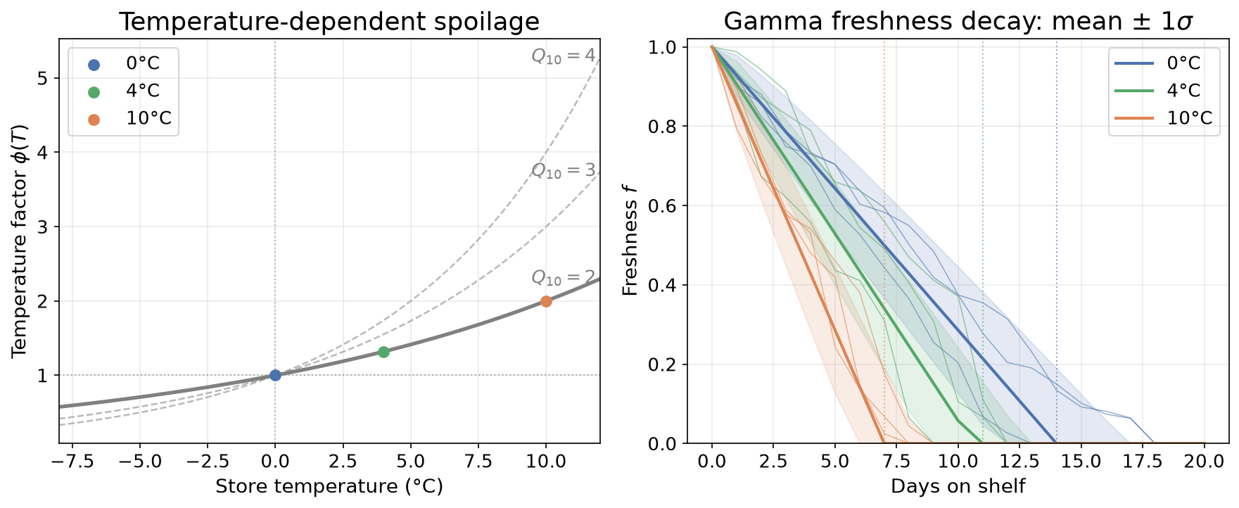
The central concept in this model is an explicit “freshness” variable, , related to physical qualities like water content but also to a shopper’s subjective preference (who wants old berries?). It starts at 1 at harvest and decreases stochastically according to a Gamma Process until it hits 0, when we call it spoiled.
The rate of freshness loss is temperature-dependent, according to the Arrhenius equation that governs temperature-dependent chemical reaction rates (such as spoilage). In food-science, this is generally phrased as a “Q10” relationship, where the spoilage rate roughly multiplies by some constant for every 10°C rise in temperature.
and set the average size and noisiness of a normal day’s loss at reference temperature ; scales that loss for whatever temperature day actually was. A day in a hot truck burns more shelf life than a day in the cooler.
In our model, we never observe freshness directly - we only infer it through indirect observation of deliveries, sales, and waste. That’s not perfectly realistic - a produce manager forms a qualitative sense of it just by looking - but that judgment doesn’t make its way into numeric form very easily in a regular grocery store, so we leave it out here.
Shipping conditions
We can think of our prior beliefs like probability distributions - maybe a produce manager has a gut instinct that there’s a 30% chance these berries are perfect on arrival, 50% alright, 20% not-so-hot. In the most primitive observation scenario, that’s all we have: a wide prior belief, uninformed by anything about this specific shipment.
The next best thing is the pack date - if the berries left the farm 2 days ago, then our expectation would be quite different than if they left 10 days ago. But if the truck’s refrigerator was broken for those whole two days, we might find ourselves quite surprised when the berries arrive. Best case, we know the full temperature history from sensor data - still not perfect (sensors fail, sit in the wrong spot, whatever), but pretty darn good.
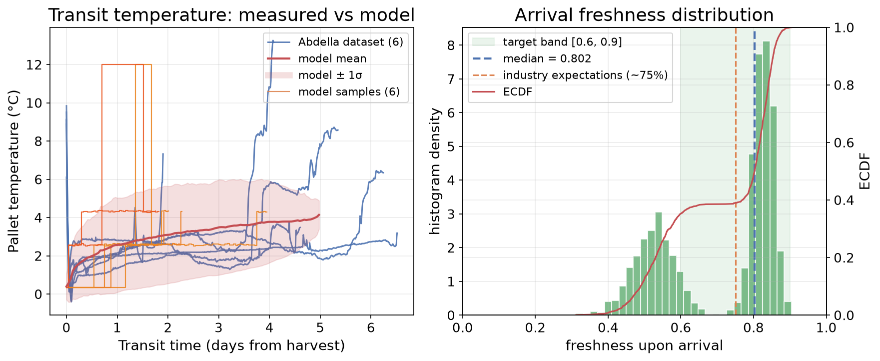
In the simulator, we generate simplistic temperature histories which are intended to very roughly resemble this real strawberry cold-chain data from Abdella et. al. Simulated trips are broken into several constant-temperature (with minor wiggles) legs of varying lengths, representing different stages of the journey from farm to store. We assume each trip is made of 3 legs. We also assume that each delivery contains 3 lots. All three lots share the last leg, since they arrive together. But they may have different early-histories, allowing for multi-echelon fulfillment schemes where different supplier shipments are combined at a distribution center before being sent to the store.
Most of the time, the generated temperatures are within reasonable cold-chain ranges (<5°C). But every so often the cold chain breaks - a stop, a door left open. The number of breaks grows with trip length; each break lasts days at a warm hold temperature before the reefer catches up again.
This piecewise-constant-ish temperature trace , when combined with the temperature sensitivity from above, defines the key summary quantity that we really care about, the cumulative thermal exposure,
We also allow for per-unit variation in the temperature history within the same shipment, with an inter-lot variation multiplier drawn from
which feeds a Gamma decay rate, as described in the previous section, to ultimately determine the arrival-freshness of each unit,
So we use the same physics to age produce in-store and in-transit, but we just assume a constant temperature in the store, and allow for more complex variation on the road.
Consumer demand
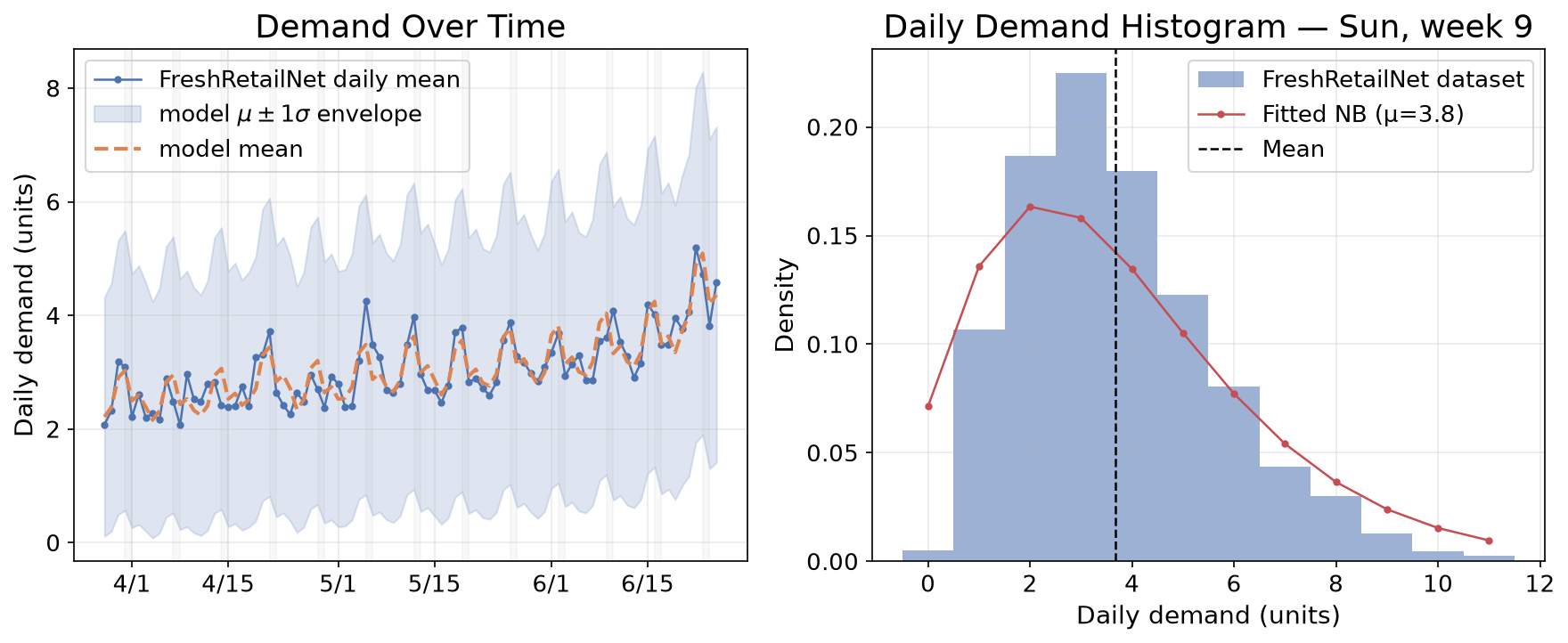
Another thing we don’t know for certain: how many blueberries people will want on any given day - probably more on July 1st than December 15th. But how much more? For this model, we assume daily demand is drawn from a Negative Binomial distribution, with a mean that varies by day-of-week and week-of-year:
fit from FreshRetailNet, an open Chinese retail-sales dataset - not blueberry-specific (product identity is anonymized), so treat it as a plausible seasonal shape rather than ground truth for blueberries.
One more piece: which specific punnet actually gets sold. Rather than a strict oldest-first or newest-first queue, we use a freshness-weighted lottery - each unit’s chance of being picked next scales as , so at every unit is equally likely, and as grows, shoppers increasingly reach for the freshest-looking punnet. Lacking any real data about this level of user preference, we arbitrarily chose to simulate some amount of shopper preference for fresher berries.
Ordering schedule
Whereas the original Afresh blog post placed same-day orders every day, we’ll use a Monday/Wednesday/Friday delivery schedule with a fixed 1-day lead-time - so orders go in on Sunday, Tuesday and Thursday for the next day’s delivery.
Economics
Obviously, each punnet of blueberries has cost to the grocer, and a sale price to the customer. The difference is the unit profit. However, if we naively maximize the per-unit profit, we’d be ignoring other considerations that are important but harder to quantify.
Of course, there are also other obvious fixed costs that the business incurs, like rent and payroll. But there are also subtler costs - how much does a stockout damage our reputation and future sales? How much time/resources does it take to deal with waste? What’s the environmental impact of food waste, and how does that impact our decisions?
In order to avoid explicitly modeling such complex topics, it’s pragmatic to assign synthetic costs to allow us to include these considerations in a simple profit-maximization strategy.
For this particular problem, we assign a per-unit stockout cost for every missed sale, and a per-unit spoilage cost for every item that we have to throw away. In our analysis, these costs are set so that a stockout is ~2x worse than spoilage, assuming that grocers prioritize customer-facing service level over silent waste.
The filter
A “filter,” in the context of data-driven decision-making, is an algorithm that infers the hidden state of a system from noisy, partial observations - it encodes our beliefs, and the uncertainty that comes with them.
Observation scenarios
We consider a variety of possibilities for what data is collected in the produce department, in order to see how different types of data can inform our decision-making process.
What a grocer is quite likely to know with decent certainty is:
- how many items were delivered
- how many were sold
We refer to this as “books only.”
Beyond that, we consider three independent observation channels:
- whether the number of units that spoil each day is recorded. Let’s assume that this is carried out by scanning each spoiled unit with a barcode scanner.
- the type of barcodes that packages carry: product-level UPC vs a 2D code carrying GTIN + lot (LGTIN). This option applies both at checkout and when recording spoilage. If LGTIN-enabled units are scanned upon spoilage, this provides more detailed information about which specific units went bad, and how long they lasted on the shelf.
- what is known about units before they arrived at the store. The base case is that nothing is known. The second option is that the pack date is known from the supplier’s ASN. The third option is that a full temperature history is available from sensor data. Knowing the pack date narrows our expectations significantly about the freshness upon delivery. A full temperature history goes even further, allowing for units which have been exposed to cold-chain interruptions to be identified clearly.
Together, these three channels define 2×2×3 = 12 possible observation scenarios. In the Results section, we analyze how each of these observation scenarios impact our understanding of the inventory, as well as our ability to act on that information.
For the sake of simplicity, we also define the following sequence of 5 scenarios which are strictly increasing in terms of information content, and might represent a realistic path that a grocer might take when upgrading their internal systems and procedures for the Sunrise 2027 era.
| Description | code_type | scan_waste | delivery_history |
|---|---|---|---|
| Books only | upc | no | none |
| + scan waste | upc | yes | none |
| + pack date | upc | yes | pack_date |
| + LGTIN | lgtin | yes | pack_date |
| + temp. history | lgtin | yes | temperature_history |
Particle filter algorithm
A Kalman filter is the classic tool for hidden state estimation, but it only works cleanly for linear systems where all the uncertainty is Gaussian. Ours is neither - freshness decays through a one-sided Gamma process, and spoilage is a hard boundary at zero, not a bell curve.
So instead we use a particle filter: maintain a population of “particles,” each one a complete, self-consistent guess about the hidden state of the world. Concretely, each particle here carries its own hypothesized freshness value for every unit currently on the shelf - not a per-lot summary, but one number per punnet, per particle. (In the implementation this is a fixed grid of lot slots × unit slots per particle, with a slot counting as alive whenever its freshness is still above zero.)
Each day, every particle ages its units forward under the same Gamma/Q10 physics as the true simulator and births new units for anything arriving that day; every particle then gets re-weighted by how well it explains whatever was actually observed (sales, reported spoilage, whatever the scenario makes visible); and once weight has concentrated onto too few particles, we resample so computation isn’t wasted on hypotheses already ruled out. The upshot: give the filter more to observe - pack dates, temperature histories, lot-level waste - and the belief narrows faster and stays tighter.
One specific risk with particle filters is that if the number of particles is too small, it’s possible that none of your beliefs are feasible, and the filter doesn’t know how to proceed. The easiest remedy is simply to increase particle count, though this in turn increases computation time.
Arrival priors
With full temperature history enabled, the filter already has a very good estimate of how fresh each unit is upon arrival. Only per-unit variability remains. When only pack-date is observed, our prior beliefs about delivery temperatures must be considered in order to infer arrival freshness. This is inherently less accurate than knowing the specific temperature conditions for a specific shipment. And when no delivery information is available, we must additionally include our prior beliefs about how long shipments take. This widens our arrival beliefs further.
Based on knowledge of the approach that the simulator uses to generate timing and temperature data for shipments, and the specific distributions/parameters in use, the filter constructs arrival beliefs based on the currently selected observation scenario. This forms the filter’s initial beliefs when new units arrive, which then get updated by subsequent observations of sales and spoilage.
The controller
Given a belief, someone still has to decide how many blueberries to order. A basic, commonly used approach, is called the “base-stock” ordering policy, where you have a target inventory level (that could be constant or demand-dependent), and whenever your stock falls below a certain “reorder-point” (or just on a regular basis), you order up to that target.
This works great for non-perishable items, but it’s sub-optimal for fresh produce because it doesn’t consider how long the current stock will last. Maybe half of your produce is about to expire the day after the shipment arrives - in that case, you should have ordered more.
We make a simple extension to the base-stock approach by replacing the current inventory level with an effective inventory,
Then, the controller’s order is given by
is effective inventory - each lot’s unit count weighted by its expected freshness, so nearly-spoiled berries count for less than fresh ones. The second term covers the pipeline: units already ordered but not yet delivered, counted at an assumed arrival freshness . Without it, the controller would re-order everything already in transit. is a demand quantile from the Negative Binomial model above: enough stock to cover demand with probability until the next delivery. scales the gap between target and effective inventory, and rounds to a whole case (you probably can’t just order 3 pints of blueberries).
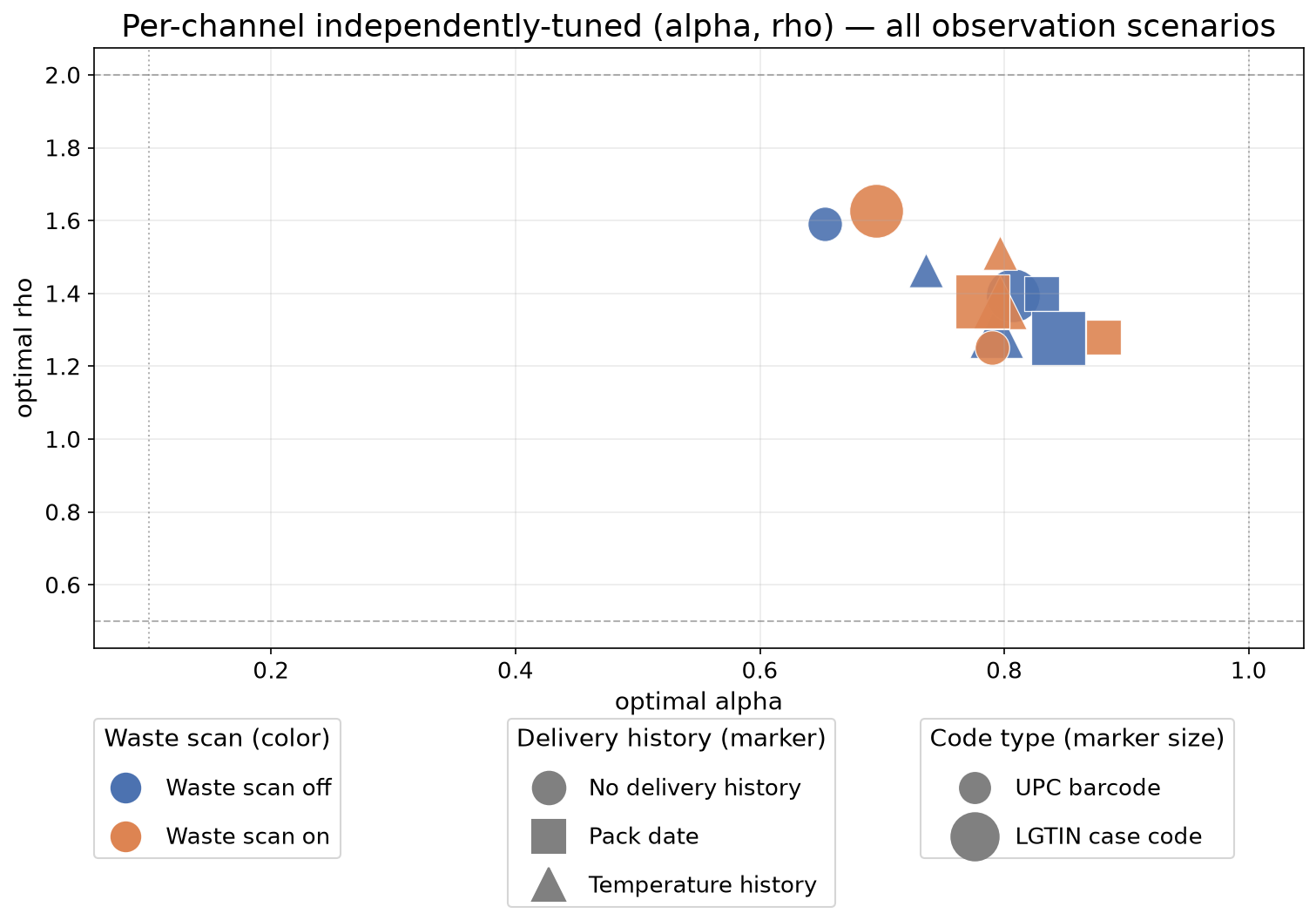
I originally thought of as a damping factor - something below 1, so orders don’t swing all the way to target in one step. In practice the tuner disagreed: every one of the 12 observation scenarios landed between 1.25 and 1.63, so the fitted controller consistently overshoots the gap rather than damping it. That’s an early hint of the over-ordering behavior we’ll come back to in the results.
The simulator
Since I don’t run a real grocery store, I built a virtual one (a small simulator). Every punnet is tracked individually - they arrive in lots but with individual freshness variance (not every punnet sat in the same spot on the truck), age via the physics above using the store’s temperature, and get sold via the freshness-weighted lottery.
One honest caveat: the simulator and the filter deliberately share the same underlying distributions for demand, arrival, and spoilage. That’s a form of cheating - real models never match reality exactly - but it isolates the question I actually care about (how much does knowing more about a well-specified system help?) rather than mixing it with model-misspecification noise.
The web interface
The filter, controller, and simulator are implemented once, in Rust, and exposed two ways from the same core crate: via WASM for the browser, and via PyO3 for Python/notebooks (and cloud batch runs on Modal). So the exact code producing this post’s numbers also runs live in your browser.
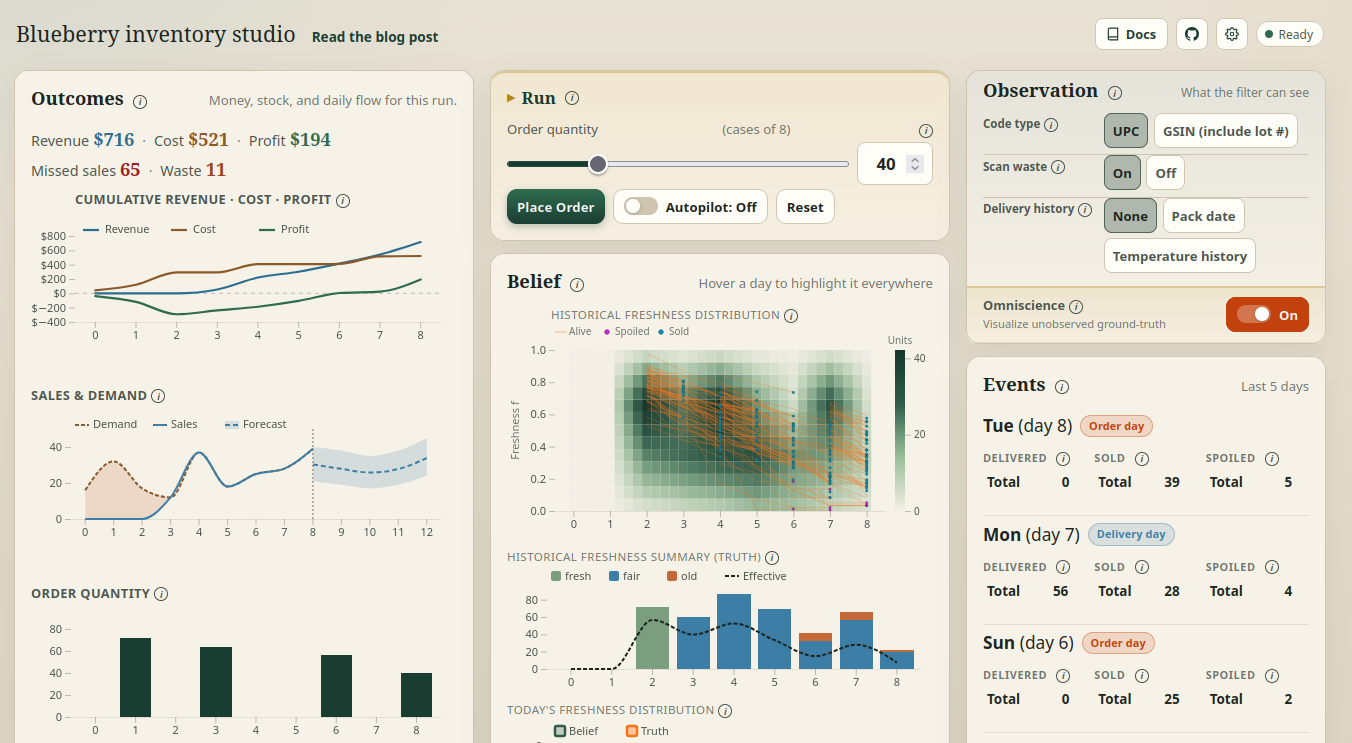
This web interface shows the filter’s freshness belief distribution evolving day by day, running P&L, sliders for (almost) every physics parameter, toggles for each observation channel, and an autopilot mode to watch different controller strategies run. You can also enable “omniscience” mode to show the raw simulator data that a real operator wouldn’t observe directly. Try it live at Blueberry Studio.
Analysis methodology
So now we attempt to address the question: what’s the value of the various observation scenarios? By comparing the filter beliefs to the simulator ground-truth, we can quantify how accurate the beliefs are. We should expect that the more detailed information produces more accurate beliefs.
Further, we can use these beliefs to drive the controller, and compare outcomes (profit, stockouts, waste) among observation scenarios.
Controller tuning
This controller has two free parameters: , the demand quantile, and , a linear factor to account for systematic over- or under-estimation of demand. It’s important to choose (“tune”) these parameters well in order for our controller to meet our objectives as well as possible.
Since is a quantile, it’s only meaningful between 0 and 1 - in practice, we search over to avoid the infinite quantile right at the boundary. Meanwhile, is an arbitrary fudge factor that could take any positive value - here, we consider values between 0.5 and 2.
| parameter | min | max |
|---|---|---|
| 0.1 | 0.9999 | |
| 0.5 | 2 |
Here, we use the Ax-platform library from Facebook to perform Bayesian Optimization in order to find the controller parameters that maximize the controller’s expected profit in the simulator. Bayesian Optimization is a great choice for optimization problems where evaluating the objective function (here: running a 30-day simulation) is computationally expensive, because the algorithm has its own internal model of the objective landscape. Most optimization steps happen against this internal model, and it only looks at the external reality infrequently in order to improve its internal beliefs.
In order to make the best possible use of the available observations, we perform this tuning independently for each of the 12 observation scenarios, allowing the controller to adapt to the particular quirks/biases of each scenario. Each scenario gets 25 BO trials, drawn from a pool of 30 seeds.
Comparing scenarios
Profit
In order to compare the controller’s profit under each observation scenario, we simply let it make ordering decisions, which affects future inventory, and in turn affect the filter beliefs in a “closed-loop”. Repeating this a few times with different random seeds, we find the distribution of profits for that scenario.
Once we have these profit distributions for all scenarios, for each seed, we calculate the ratio of profit between each observation scenario and the “books-only” baseline. This yields a distribution of profit ratios for each scenario.
Filter beliefs
To compare the filter under these scenarios, we’d like to provide a more even comparison, by ensuring that for a given seed, the filter is forming its beliefs based on the exact same observations each time. Therefore, we use an “open-loop” approach, where the controller is not used - instead, a fixed order schedule is used across scenarios.
Calculating the filter accuracy is also a bit more complex. Whereas profit is a single number per episode, filter belief and freshness ground-truth are both probability distributions for each day. One approach we use is to calculate the Wasserstein distance (a.k.a. earth-mover metric), which quantifies the difference between two probability distributions. We take the average over all days to get one number per (seed, scenario). Then, like profit, we calculate the same-seed ratios compared to the books-only baseline to get a final error distribution for the filter’s full freshness beliefs.
Alternatively, we can just look at the filter’s daily (posterior mean) count of units on the shelf (disregarding freshness), and compare that to the simulator ground-truth, and take the mean absolute error (MAE) over all days. Like before, we then calculate MAE ratios of each scenario vs the baseline across all seeds to produce distribution of aggregated count errors.
Results
So when we do all of that, here’s what we see:
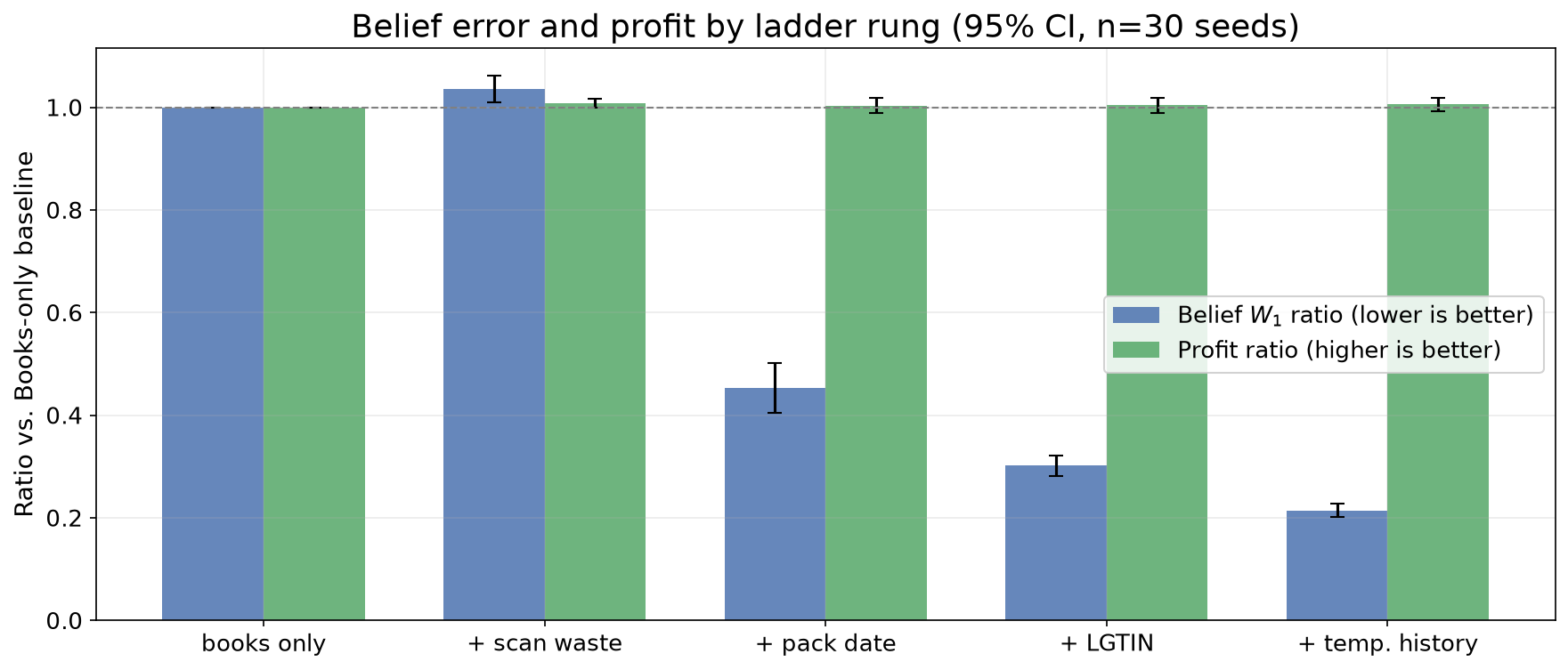
| Observation scenario | Belief ratio (95% CI) | Profit ratio (95% CI) |
|---|---|---|
| Books only | 1.000 (baseline) | 1.000 (baseline) |
| + scan waste | 1.036 ± 0.026 | 1.009 ± 0.008 |
| + pack date | 0.453 ± 0.048 | 1.003 ± 0.015 |
| + LGTIN | 0.301 ± 0.019 | 1.004 ± 0.014 |
| + temp. history | 0.214 ± 0.013 | 1.006 ± 0.014 |
Belief improves pretty steadily as we add more nuanced observations, but profit stays totally flat - all profits are within 1% of the baseline. In other words, our controller doesn’t convert better beliefs into higher profit at all.
Pack date alone cuts belief error by more than half - the single biggest jump on the ladder. Lot-level scanning and full temperature history each buy further real, if smaller, gains on top. Daily waste counts alone, with no delivery information, barely move the needle, and might even make things slightly worse.
Freshness and profit
Let’s dig in further by looking at all 12 observation scenarios.
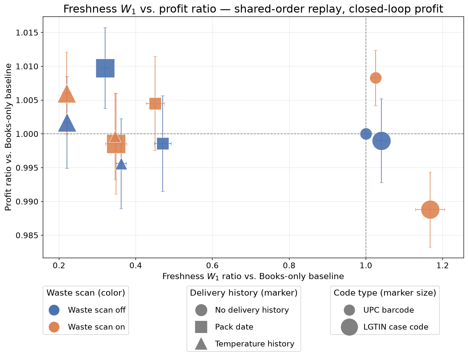
Looking at the figure above, the first thing you’ll notice is that all of the circles are on the right side - this is the same jump from the bar chart above, where knowing the pack date provides a huge boost to freshness belief accuracy.
Another thing that you might notice if you really squint your eyes is a slight downward trend - an indication that better beliefs lead to more profit. But as mentioned before, all the profit values are within 1% of the baseline, so we’re pretty much counting pennies.
Freshness and count
Now, let’s compare the two belief error metrics we’ve discussed - unit count error and freshness .
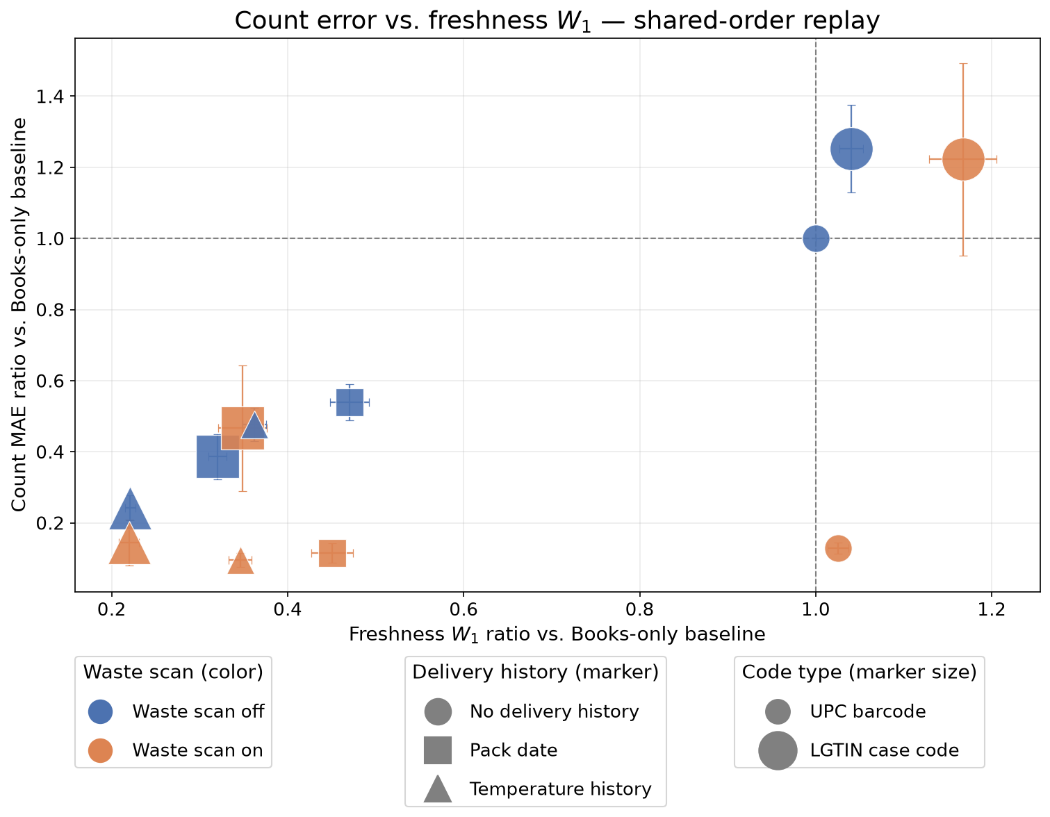
Remember above in the scenario ladder bar chart where adding waste scanning made the freshness belief slightly worse than the baseline? Well, here you can see in detail that while waste scanning doesn’t really help the accuracy of the filter’s freshness distribution, it does more for the count accuracy than any other observation channel. Notice all of the orange points along the bottom of the figure - adding waste scanning almost always gives you a highly accurate view of the number of units currently on the shelf, regardless of the other channels.
A sad controller
So why is the controller so indifferent to belief accuracy? Well, one possibility is that it really doesn’t matter how accurate your inventory beliefs are. I don’t think that’s true in general, but it might be true in this particular situation - that given this particular set of physical and economic parameters, the baseline belief is already good enough. In particular, the objective punishes stockouts far harder than spoilage. Throwing a punnet away costs the 2.70 margin we forgo plus the 5.20, or about 4.3x more. Under those economics, over-ordering is a cheap way to roughly maximize profit, even if it’s not Pareto-optimal when considering stockout and waste as separate objectives. Or, it could be that since blueberries last about 10 days on a 4°C shelf, while orders are placed every few days, a freshness-aware controller doesn’t buy you that much (although the original Afresh blog post seems to be arguing otherwise). Perhaps the 1-day lead-time we use also makes it quite easy to order well, even without great information.
I think the more likely answer, though, is that the controller is too simplistic and short-sighted. Every time it places an order, it only considers the current mean freshness and the demand over the protection interval (the next few days, until the subsequent order arrives). Given that the shelf life of berries is significantly longer than that horizon, the controller might just not be able to take into account the time frame over which spoilage really matters.
I experimented briefly with a few other controller designs that didn’t end up improving much. One was a “rollout” controller that simulates future outcomes over a finite horizon using the default simplistic controller and chooses the next move that maximizes profit over that horizon. But it’s still quite limited by the default controller it’s based on, and it ended up just increasing the computational overhead significantly without moving the profit hardly at all, even under careful tuning of the rollout parameters. Another approach I attempted was a controller that more properly calculates the actual Gamma decay and aims to maintain a desired service-level (stockout rate) over the protection interval. But it didn’t improve profit either, likely because it was also short-sighted, only considering spoilage over the next few days, whereas it’s probably necessary to look farther into the future.
So overall, I would chalk this up to an inadequate controller or easy store conditions, rather than a general statement that better beliefs don’t improve outcomes.
Can you do better?
So rather than continuing to experiment on my own with other controllers, I thought I’d take a more collaborative route and enlist your support. Do you have a better idea? Can you design a controller that better leverages accurate inventory beliefs and turns them into profit?
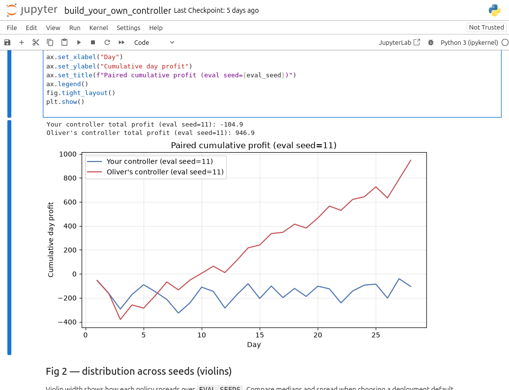
Everything above - filter, simulator, belief state - is available as a fixed harness in notebooks/build_your_own_controller.ipynb. You get a ControllerContext every day and implement one function, order(ctx) -> int. A worked example comes with it - a naive fixed-target base-stock controller - benchmarked against my policy on the same paired seeds, with cumulative-profit and across-seed distribution charts included. If you’d rather start from something that learns, TabularQLearningController in blueberries_voi.controller.starter is a small ε-greedy Q-learner over (weekday, on-hand bin) that plugs into the same harness.
This post’s title asked what you’d do if you knew more about your blueberries. Here’s your chance to actually answer that: clone the repo, write your own order(ctx), and see if you can beat my controller on my own benchmark. Tell me about it in the comments. I would love to see what you come up with!
Conclusion
Well, this has been a fun opportunity to dive deep into a mathematical rabbit hole, perhaps deeper than necessary. Whenever attempting any kind of mathematical analysis of the real world, complexity can grow quickly! As much as I’d like to continue digging and refining until all of the results are pristine, I think I’d better leave it here for now.
The one-line summary is that the more detailed information enabled by Sunrise 2027 can definitely help decision makers keep better track of their inventory. Whether that can be translated cleanly into profits will have to be a question for another day.
Directions for future work
- A better controller - probably reinforcement learning / approximate dynamic programming
- Correctness verification - I did some basic sanity checks on the codebase (interactive UIs really help to surface obvious issues), but I would want to do a much more thorough verification of all of the algorithms and parameter choices before any of this touches a real decision.
- A Pareto frontier, not one tuned point. The controller tuning currently just performs single-objective profit optimization, but a multi-objective approach could be taken. A Pareto frontier of controller parameters over (stockouts, spoilage), and could be exposed to the user at runtime to allow them to use their own preferences to navigate the tradeoffs.
- Subjective freshness as an observation channel - a produce associate’s qualitative “these look tired” assessment, captured regularly, could plausibly be folded into the filter alongside the barcode-driven channels here.
- Investigate specific situations where fine-grained data is most helpful - it’s one thing to look at average profit under normal circumstances, but it would also be worth looking into specific rare situations. How does lot-level temperature information help you identify and respond when a bad shipment comes in? Maybe certain produce items are more sensitive to better data than others, either because of their spoilage physics, or their supply-chain properties.
- Account for faulty observations - in the real world, miscounts, theft, and data-entry errors are important considerations that the filter should take into account
- Dynamic freshness-aware pricing - this whole post has dealt only with the question of how much to order. But an even bigger open question is “how does lot-level freshness information support dynamic freshness-based pricing?” This is the large-scale, data-driven analog to the half-off “distressed produce” shelf at the local co-op.
Appendix: parameter reference
For readers who want the exact numbers behind the plots above, here’s a consolidated reference of the model parameters discussed in this post.
Click to show parameter values
Freshness & spoilage physics
| Parameter | Symbol | Value |
|---|---|---|
| Reference shelf life | 14 days | |
| Q10 temperature factor | 2.0 | |
| Reference temperature | 0 °C | |
| Store temperature | 4 °C | |
| Gamma shape | 2.0 | |
| Gamma scale | ≈0.0357 | |
| Freshness-weighted picking exponent | 0.5 |
Cold-chain / shipping
| Parameter | Symbol | Value |
|---|---|---|
| Break rate | 0.08 / day | |
| Mean break duration | 0.5 days | |
| Break (warm-hold) temperature | 12 °C | |
| Inter-lot position noise | 0.08 |
Consumer demand
| Parameter | Symbol | Value |
|---|---|---|
| Baseline daily demand mean | 30 units | |
| Demand variance-to-mean ratio | 2.0 |
Ordering
| Parameter | Value |
|---|---|
| Delivery days | Mon, Wed, Fri |
| Order (placement) days | Sun, Tue, Thu |
| Lead time | 1 day |
| Case size | 8 units |
Economics
| Parameter | Value |
|---|---|
| Sell price | $4.50 / unit |
| Purchase cost | $1.80 / unit |
| Unit margin | $2.70 / sale |
| Waste (spoilage) cost | $1.20 / unit |
| Stockout penalty | $2.50 / lost sale |
Particle filter
| Parameter | Symbol | Value |
|---|---|---|
| Particle count | 200 | |
| Lot slots per particle | 50 | |
| Unit slots per lot | 15 | |
| Freshness bins (belief wire) | 30 |
Parting words
All of these results should be considered preliminary - they are based on a certain set of conditions and assumptions which may not reflect the realities of a particular store.
If you’re interested in the specific questions addressed in this article, or similar problems in other domains, please Hire Me! I’m currently open to contract or full-time roles, either remote or in-person (willing to relocate, preferably US West Coast). I would love to collaborate with smart folks working on interesting, meaningful problems, especially ones that contribute to creating a future where humanity makes it through our current polycrisis, and we learn to live in harmony with each other and this beautiful Earth.
As the famous mathematician Paul Erdős was known to say when arriving uninvited at the doorstep of a collaborator, “my brain is open!”
Thanks for reading!
Take good care,
Oliver